NESSUS Efficient Global Reliability Analysis [1]
Efficient Global Reliability Analysis (EGRA) is a surrogate based reliability analysis method. EGRA locates multiple points (also called training points) on the limit state throughout the random variable space and uses these points to construct a Gaussian process model that provides a global approximation for the entire limit state. An effective model is created with a minimal number of samples by focusing the samples only in the region of the limit state. This model is then used as an inexpensive surrogate to provide function evaluations in a sampling method to perform probability integration which leads to highly accurate probability estimates. EGRA performs an iterative process based on the expected feasibility function (EFF). The EFF is used to select the location at which a new training point must be added to the Gaussian process model by maximizing the expectation that the point lies on the limit state contour. A point could be expected to lie on the limit state contour if its predicted value is near the limit state value, or if the uncertainty in its prediction is such that there is a significant probability of its true value being near the limit state value. The general procedure of EGRA is as follows:
- 1. Build an initial Gaussian Process model of the response function.
- 2. Find the point that maximizes EFF. If the EFF value at this point is sufficiently small, stop.
- 3. Evaluate the response function at the point where the EFF is maximized. Update the Gaussian process model using this new point. Go to Step 2.
EGRA has the potential to produce very accurate probabilities of failure just like sampling methods while being as efficient as the MPP based methods, even for nonlinear limit states, using a small number of samples. The training points selected by EGRA are added from the tails of the distribution of design variables and thus providing good estimate of the limit state function. EGRA does not have limitations that the other gradient based methods face. EGRA is highly efficient and accurate method for design variables less than 10, higher number of variables makes the process computationally expensive. Once the training points are evaluated on the original model, EGRA performs sampling on the response surface so for sometime it may look like the Data Explorer is showing no new model evaluations, that is the sign that the sampling procedure is taking place. The picture shows the various option/parameters that can be set for EGRA.
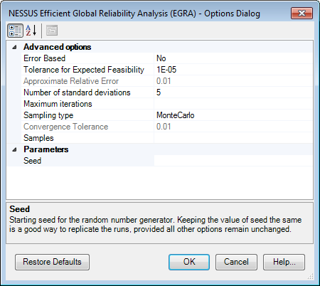
Control Parameters
| Name | Default Value | Description |
|---|---|---|
| Seed | Starting seed for the random number generator. Keeping the value of seed the same is a good way to replicate the same results between different runs, provided all other options remain unchanged. The option accepts integer values only. | |
| Error Based | No | Indicates whether or not convergence is based on estimated relative error in the failure probability. |
| Tolerance for Expected Feasibility | 1E-05 | When Error Based is set to 'No', this is the tolerance value that governs when the method will stop adding additional 'training points' to the response surface model. If this value is increased it may reduce the amount of samples used at the cost of a less accurate response surface model and thus less accurate results. Thus this option controls how many samples are actually taken on the original model. Option value should be greater than 0. |
| Approximate Relative Error | 0.01 | When Error Based is set to "Yes", this is the relative tolerance used on the probability under computation. Note that this is only an approximate error tolerance. Using this option can add significant computational overhead. Option value should be greater than 0. |
| Number of Standard Deviations | 5 | This option sets the number of standard deviations the method will search over. This option governs how far into the tails of the design variables distribution will the method search to add new points to the response surface model (training points). EGRA uses EFF to make sure the process of adding points is efficient and optimum. The default value of 5 is good, increasing it could lead to longer computations. The method only allows positive values for this option. 8.29 is the upper limit on the options value, values greater than it will generate a warning in the Messages tab. |
| Maximum Iterations | This option controls the convergence of the method. The maximum number of iterations to be performed after the basic (n+1)*(n+2)/2 evaluations where n is the number of design variables. The method performs one evaluation per iteration. If the method ends because of the value specified by this option, a warning will be listed in 'Messages' tab. By default this option is left blank but the value it uses is 50*n . The advantage of using the default value is that it allows the method to converge on its own. Thus in default case the maximum total number of evaluations will be [(n+1)*(n+2)/2 + 50*n]. | |
| Sampling Type | Monte Carlo |
This option is used to select the type of sampling method to be used on the response surface model to compute the probability of failure. The types are:
|
| Convergence Tolerance | 0.01 | This option is only used when the Sampling Type used is Multimodal Adaptive Importance Sampling. This is the convergence tolerance used by the sampling method to stop. The option should have a value preferably within 0 and 1. |
| Samples | 1,000,000 or 1,000 | This option is optional. It controls the number of samples that will be used when sampling the response surface model. For the Multimodal Adaptive Importance Sampling method, this specifies the number of samples per iteration but for all the other sampling methods this option specifies the total number of samples to be used. The default sample size is 1,000,000 for Monte Carlo and LHS. The default sample size is 1,000 for Multimodal Adaptive Importance Sampling and Multimodal Importance Sampling. Sample size should not be very small as it may lead to higher error in the estimated probability. |
Expected Feasibility Function
The expected feasibility function is used to select the location at which a new training point should be added to the Gaussian Process model. It does this by calculating the expectation that the true value of the response is expected to satisfy the equality constraint  (i.e. it lies on the limit state) based on the expected values and variances predicted by the current GP model. An important feature of the EFF is that it provides a balance between exploiting areas of the search space where the limit state has previously been found, and exploring the areas of the search space where the uncertainty is high. At any point in the design space, the GP prediction is a Gaussian distribution, defined as:
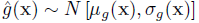
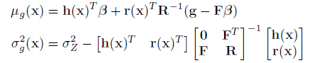
where the mean and variance are defined as:
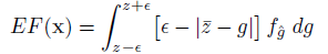
EGRA defines the expected feasibility function as:

where the epsilon term is used to focus the search in the immediate vicinity of the response threshold. Thus the expectation can be calculated as:
where g denotes a realization from the distribution  (pdf). Allowing z+ and z- to denote the upper and lower integral bounds respectively from previous equation, analytical expression is as follows:
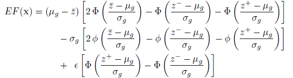
where epsilon is proportional to the standard deviation of the GP predictor. In this case, z+ and z-, mean, standard deviation and epsilon are all functions of the location x, while z-bar is constant. EFF provides a balance between exploration and exploitation.
Efficient Global Reliability Analysis Algorithm
Process of the EGRA algorithm:
- 1. Small number of samples generated from true response function using Latin Hypercube Sampling technique. The samples span over design variable bounds over 5 standard deviations by default.
- 2. Construct an initial Gaussian process model from these samples.
- 3. Find the point with maximum expected feasibility. A global optimizer DIRECT (DIviding RECTangles) is used. This algorithm follows a similar logic like that of DAKOTA Coliny DIRECT or DAKOTA NCSU DIRECT. If the maximum expected feasibility is less than Tolerance for Expected Feasibility, the model has converged. Go to Step 6.
- 4. Evaluate true response function at this point (this is a training point).
- 5. Add this new sample to previous set and build a new GP model. Go to step 3.
- 6. The resulting GP model is used to calculate probability using any sampling method.
References:1. NESSUS Theoretical Manual, February 17, 2012, Section 9.1